Fitting Piecewise Growth Models in R

July 29, 2014

This is a simple walkthrough on how to specify a piecewise linear growth model in R using the lme4 package. Just as a quick outline, I will start with a simple linear growth pattern, then extend the logic to look at piecewise growth.

Plain old linear growth

Here is an example just simulating linear growth. We will assume that everyone follows the same linear pattern over time, with some random variability around both the intercept and slope parameters.

Step 1: Simulate data

For this example, I’m simulating 100 participants with 6 timepoints each. The intercept is 10, while the slope is -2. The intercept and slope will also be positively correlated. This indicates that participants who start higher (i.e., a higher intercept) tend to have more positive change, compared to those who start lower (i.e., a lower intercept).

require(MASS) 
require(lme4)
require(ggplot2)

set.seed(42)

nPart = 100
nTime = 6

intSlope <- mvrnorm(nPart, mu = c(10, -2),
                    Sigma = matrix(c(4, 1, 1, 2), nrow = 2))

myData <- expand.grid(ID = 1:nPart, Time = 0:(nTime - 1))
myData <- myData[order(myData$ID, myData$Time), ]

score <- c(NA)

for(i in 1:nrow(myData)){
  
  df <- myData[i,]
  score[i] <- intSlope[df$ID, 1] + df$Time * intSlope[df$ID, 2] + rnorm(1)
  
}

myData$Score <- score

head(myData)

##     ID Time     Score
## 1    1    0   5.91669
## 101  1    1   3.75189
## 201  1    2   0.08993
## 301  1    3  -3.52136
## 401  1    4 -11.45727
## 501  1    5 -15.73077

Step 2: Plot the data

You can see that I simulated the dataset to be in long format. I also started Time at 0, so the intercept would be interpreted as the mean of the first measure. Using spaghetti plots, we can visualize what the simulated data look like.

ggplot(aes(x = Time, y = Score), data = myData) +
  geom_line(aes(group = ID), color = "gray") + 
  geom_smooth(aes(group = 1), method = "lm", size = 3, color = "red", se = FALSE) +
  theme_bw()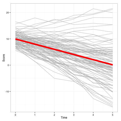

center

We see that the intercept is around 10, with a decreasing slope around 2. This should not be a surprise, given those are the parameters we simulated.

Step 3: Build the model

For this example, we are going to use lme4 to create a mixed-effects model. Here we have observations nested within individual. In this case, time will be a level-1 predictor. We will also allow both intercept and time to vary systematically around our intercept and slope estimates (and this variation between intercept and slope also has a covariance).

In this output, we are first presented with random effects. This tells us that the intercept has a variance of around 4 and the slope for Time has a variance of around 2. Again, this is similar to what we simulated. Next are the fixed effects, and we capture the original parameters quite accurately.

linearModel <- lmer(Score ~ 1 + Time + (1 + Time | ID),
                    data = myData)

summary(linearModel)

## Linear mixed model fit by REML ['lmerMod']
## Formula: Score ~ 1 + Time + (1 + Time | ID)
##    Data: myData
## 
## REML criterion at convergence: 2373
## 
## Scaled residuals: 
##     Min      1Q  Median      3Q     Max 
## -2.6307 -0.5577 -0.0233  0.5739  2.1918 
## 
## Random effects:
##  Groups   Name        Variance Std.Dev. Corr
##  ID       (Intercept) 4.03     2.01         
##           Time        1.81     1.35     0.48
##  Residual             1.01     1.01         
## Number of obs: 600, groups: ID, 100
## 
## Fixed effects:
##             Estimate Std. Error t value
## (Intercept)    9.931      0.214    46.5
## Time          -1.962      0.137   -14.3
## 
## Correlation of Fixed Effects:
##      (Intr)
## Time 0.398

Piecewise linear growth

Now, here is an example simulating two growth patterns.

Step 1: Simulate data

In this case, I’m still simulating 100 participants with 6 timepoints. However, this time I will assume no growth for the first 3 time points, followed by a decline in the next 3 time points. The intercept will still be 10, and the slope for the second piece will still be -2. To make things a little easier, no correlation between intercept and either slope will be simulated.

intSlopeNew <- mvrnorm(nPart, mu = c(10, 0, -2),
                       Sigma = matrix(c(4, 0, 0, 0, 1, 0, 0, 0, 2),byrow = TRUE, nrow = 3))

myDataNew <- data.frame(ID = rep(1:nPart, each = 6),
                        Time = 0:(nTime - 1),
                        Time1 = c(-2, -1, 0, 0, 0, 0),
                        Time2 = c(0, 0, 0, 1, 2, 3))

scoreNew <- c(NA)

for(i in 1:nrow(myData)){
  
  df <- myDataNew[i,]
  score[i] <- intSlopeNew[df$ID, 1] + df$Time1 * intSlopeNew[df$ID, 2] +
              df$Time2 * intSlopeNew[df$ID, 3] + rnorm(1)
  
}

myDataNew$Score <- score

head(myDataNew, n = 12)

##    ID Time Time1 Time2  Score
## 1   1    0    -2     0  6.077
## 2   1    1    -1     0  8.049
## 3   1    2     0     0 10.843
## 4   1    3     0     1 10.599
## 5   1    4     0     2 10.642
## 6   1    5     0     3  9.790
## 7   2    0    -2     0 10.296
## 8   2    1    -1     0 10.069
## 9   2    2     0     0 12.577
## 10  2    3     0     1 10.015
## 11  2    4     0     2  6.023
## 12  2    5     0     3  5.082

Step 2: Plot the data

This time, I have two time variables: Time1 and Time2. As you can imagine, Time1 represents the first growth pattern, while Time2 represents the second. The intercept is the score when both time variables are 0, which is the third datapoint for each person.

ggplot(aes(x = Time, y = Score), data = myDataNew) +
  geom_line(aes(group = ID), color = "gray") + 
  geom_smooth(aes(group = 1), size = 3, color = "red", se = FALSE) +
  theme_bw()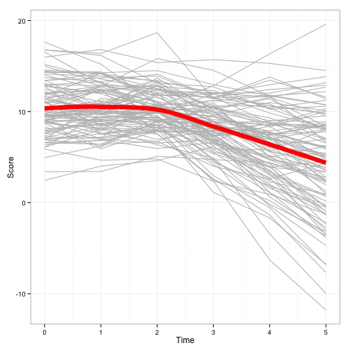

center

Step 3: Build the model

Model building for this model seems like it should be complex, but it really is just as simple as including the second time variable as both a fixed and random effect. From the output, we see the variance components for each random effect. These are interpreted the same: they tell us how variable our sample is with regard to each component. The fixed-effects are about 10 for our intercept, around 0 for the first slope, and -2 for the second slope. Just as was simulated, this model tells us the data seem to be relatively stable throughout the baseline, then declining after baseline. Including additional predictors/interactions with time follow logically from the above example.

plgModel <- lmer(Score ~ 1 + Time1 + Time2 + (1 + Time1 + Time2 | ID),
                 data = myDataNew)

summary(plgModel)

## Linear mixed model fit by REML ['lmerMod']
## Formula: Score ~ 1 + Time1 + Time2 + (1 + Time1 + Time2 | ID)
##    Data: myDataNew
## 
## REML criterion at convergence: 2492
## 
## Scaled residuals: 
##     Min      1Q  Median      3Q     Max 
## -2.6278 -0.4664  0.0103  0.5049  2.9113 
## 
## Random effects:
##  Groups   Name        Variance Std.Dev. Corr       
##  ID       (Intercept) 4.529    2.128               
##           Time1       0.854    0.924    -0.05      
##           Time2       2.805    1.675     0.07  0.16
##  Residual             1.050    1.025               
## Number of obs: 600, groups: ID, 100
## 
## Fixed effects:
##             Estimate Std. Error t value
## (Intercept)  10.2517     0.2275    45.1
## Time1        -0.0663     0.1139    -0.6
## Time2        -1.9445     0.1732   -11.2
## 
## Correlation of Fixed Effects:
##       (Intr) Time1 
## Time1  0.115       
## Time2 -0.005  0.042

Wicked Good Data